Mode Selection
The mode selection module is paramount to the computational efficiency of this model. Below we show how we perform this selection operation by providing a trajectory to the ModeSelector module and obtaining only strongly-contributing modes.
Mode selection by power contribution
[1]:
import numpy as np
import matplotlib.pyplot as plt

import few

from few.trajectory.inspiral import EMRIInspiral
from few.trajectory.ode import SchwarzEccFlux
from few.amplitude.ampinterp2d import AmpInterpSchwarzEcc
from few.utils.ylm import GetYlms
from few.utils.modeselector import ModeSelector

# tune few configuration
cfg_set = few.get_config_setter(reset=True)

# Uncomment if you want to force CPU or GPU usage
# Leave commented to let FEW automatically select the best available hardware
#   - To force CPU usage:
# cfg_set.enable_backends("cpu")
#   - To force GPU usage with CUDA 12.x
# cfg_set.enable_backends("cuda12x", "cpu")

cfg_set.set_log_level("info");
[2]:
# first, lets get amplitudes for a trajectory
traj = EMRIInspiral(func=SchwarzEccFlux)

# parameters
m1 = 1e5
m2 = 1e1
a = 0.0 # Schwarzschild
p0 = 10.0
e0 = 0.7
theta = np.pi / 3.0
phi = np.pi / 2.0

t, p, e, x, Phi_phi, Phi_theta, Phi_r = traj(m1, m2, 0.0, p0, e0, 1.0)

amp_module = AmpInterpSchwarzEcc()
ylm_gen = GetYlms()

# select modes

mode_selector = ModeSelector(
    amp_module,
    ylm_generator=ylm_gen,  # optional, this is the default choice
    force_backend="cpu"
)

mode_selection_threshold = 1e-2  # target mismatch between reduced and full mode content waveforms

(teuk_modes_r, ylms_r, ls_r, ms_r, ks_r, ns_r) = mode_selector(
    t,
    a,
    p,
    e,
    x,
    theta,
    phi,
    mode_selection_threshold=mode_selection_threshold  # this can also be provided to ModeSelector() on instantiation
)

(teuk_modes, ylms, ls, ms, ks, ns) = mode_selector(
    t,
    a,
    p,
    e,
    x,
    theta,
    phi,
    mode_selection = "all",  # this can also be provided to ModeSelector() on instantiation
)

print(
    "We reduced the mode content from {} modes to {} modes.".format(
        teuk_modes.shape[1], teuk_modes_r.shape[1]
    )
)
We reduced the mode content from 3843 modes to 59 modes.
Mode selection by noise-weighted power contribution
Modes can also be weighted by a Power Spectral Density (PSD) function from your favorite sensitivity curve. This ensures that the target mismatch is with respect to the PSD that will be used in (for example) parameter estimation.
Note: FEW assumes that the PSD function is valid over all frequencies, and will evaluate it at particularly high frequencies for the highest-order modes in the model. Ensure that the PSD remains well-behaved at all frequencies (or simply pad high-frequency inputs with a large number to zero-out these contributions) for accurate results.
[3]:
from few.summation.interpolatedmodesum import CubicSplineInterpolant
from few import get_file_manager
# produce sensitivity function
noise = np.genfromtxt(get_file_manager().get_file("LPA.txt"), names=True) # LISA PSD
f, PSD = (
np.asarray(noise["f"], dtype=np.float64),
np.asarray(noise["ASD"], dtype=np.float64) ** 2,
)
sens_fn = CubicSplineInterpolant(f, PSD)
# select modes with noise weighting
# provide sensitivity function kwarg
mode_selector_noise_weighted = ModeSelector(
amp_module,
ylm_generator=ylm_gen, # optional, this is the default choice
sensitivity_fn=sens_fn
)
# we need the orbital frequencies when noise-weighting
# these can be computed from the trajectory output efficiently
freqs = traj.inspiral_generator.eval_integrator_derivative_spline(t, order=1)[:,3:6] / 2 / np.pi
online_mode_selection_args = dict(
f_phi = freqs[:,0],
f_theta = freqs[:,1],
f_r = freqs[:,2],
)
(teuk_modes_r_nw, ylms_r_nw, ls_r_nw, ms_r_nw, ks_r_nw, ns_r_nw) = mode_selector_noise_weighted(
t,
a,
p,
e,
x,
theta,
phi,
online_mode_selection_args=online_mode_selection_args,
mode_selection_threshold=mode_selection_threshold # this can also be provided to ModeSelector() on instantiation
)
print(
"We reduced the mode content from {} modes to {} modes when using noise-weighting.".format(
teuk_modes.shape[1], teuk_modes_r_nw.shape[1]
)
)
# plot histogram of modes
plt.figure()
plt.hist(ns_r_nw, bins=100, label="n")
plt.xlabel("n")
plt.ylabel("Number of radial modes")
plt.show()
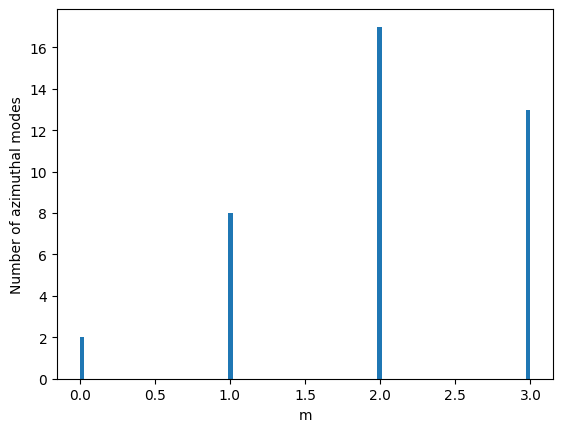
plt.figure()
plt.hist(ms_r_nw, bins=100, label="n")
plt.xlabel("m")
plt.ylabel("Number of azimuthal modes")
plt.show()
(CubicSplineInterpolant) Warning: New t array outside bounds of input t array. These points are filled with edge values.
We reduced the mode content from 3843 modes to 40 modes when using noise-weighting.

Compare the two waves with and without noise-weighting
[4]:
from few.waveform import FastSchwarzschildEccentricFluxBicubic
from few.utils.utility import get_mismatch


noise_weighted_mode_selector_kwargs = dict(sensitivity_fn=sens_fn)

inspiral_kwargs = {
    "DENSE_STEPPING": 0,  # we want a sparsely sampled trajectory
}

# keyword arguments for inspiral generator (RomanAmplitude)
amplitude_kwargs = {
}

# keyword arguments for Ylm generator (GetYlms)
Ylm_kwargs = {
    "include_minus_m": False  # if we assume positive m, it will generate negative m for all m>0
}

# keyword arguments for summation generator (InterpolatedModeSum)
sum_kwargs = {
    "pad_output": False,
}

few_base = FastSchwarzschildEccentricFluxBicubic(
    inspiral_kwargs=inspiral_kwargs,
    amplitude_kwargs=amplitude_kwargs,
    Ylm_kwargs=Ylm_kwargs,
    sum_kwargs=sum_kwargs,
)

few_noise_weighted = FastSchwarzschildEccentricFluxBicubic(
    inspiral_kwargs=inspiral_kwargs,
    amplitude_kwargs=amplitude_kwargs,
    Ylm_kwargs=Ylm_kwargs,
    sum_kwargs=sum_kwargs,
    mode_selector_kwargs=noise_weighted_mode_selector_kwargs,
)

m1 = 1e6
m2 = 1e1
p0 = 12.0
e0 = 0.3
theta = np.pi / 3.0
phi = np.pi / 4.0
dist = 1.0
dt = 10.0
T = 0.001

wave_base = few_base(m1, m2, p0, e0, theta, phi, dist=dist, dt=dt, T=T, mode_selection_threshold=1e-2)
wave_weighted = few_noise_weighted(
    m1, m2, p0, e0, theta, phi, dist=dist, dt=dt, T=T, mode_selection_threshold=1e-2
)

plt.plot(wave_base.real, label="base")
plt.plot(wave_weighted.real, ls='--', label="noise-weighted")
plt.legend()
print("mismatch:", get_mismatch(wave_base, wave_weighted))
print("base modes:", few_base.num_modes_kept)
print("noise-weighted modes:", few_noise_weighted.num_modes_kept)
(CubicSplineInterpolant) Warning: New t array outside bounds of input t array. These points are filled with edge values.
mismatch: 0.013279647100721492
base modes: 12
noise-weighted modes: 17

Specific mode selection
The user can also select a specific set of modes to use in the waveform.
[5]:
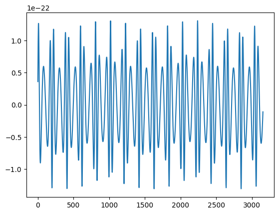
# l = 2, m = 2 wave
specific_modes = [(2, 2, 0, n) for n in range(-30, 31)]

wave_22 = few_base(
    m1, m2, p0, e0, theta, phi, dist=dist, dt=dt, T=T, mode_selection=specific_modes
)

plt.plot(wave_22.real)

print("mismatch with full wave:", get_mismatch(wave_22, wave_base))
(ModeSelector) Warning: Mode selection is large. Instantiate class with mode selection rather than providing it at call time for better performance.
mismatch with full wave: 0.04028675532908721
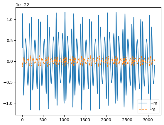
Turn off \((-m, -k, -n)\) modes
By default, symmetry is used to generate \((-m, -k, -n)\) modes from their corresponding \((m, k, n)\) counterparts. To disable this behaviour, provide False to the include_minus_mkn kwarg. This only affects the waveform when mode_selection is a list of specific modes.
As some checks are performed on mode_selection during waveform evaluation, if the same mode content for many waveforms is required, it can be more efficient to provide this list of modes to mode_selector_kwargs when instantiating the waveform generator object.
[6]:
%matplotlib inline
# l = 2, m = 2 wave without m = -2
specific_modes = [(2, 2, 0, n) for n in range(-30, 31)]

specific_modes_minus_m = [(2, -2, 0, n) for n in range(-30, 31)]

wave_22_pos_m = few_base(
    m1,
    m2,
    p0,
    e0,
    theta,
    phi,
    dist=dist,
    dt=dt,
    T=0.001,
    mode_selection=specific_modes,
    include_minus_mkn=False,
)

wave_22_minus_m = few_base(
    m1,
    m2,
    p0,
    e0,
    theta,
    phi,
    dist=dist,
    dt=dt,
    T=0.001,
    mode_selection=specific_modes_minus_m,
    include_minus_mkn=False,
)

plt.plot(wave_22_pos_m.real, label="+m")
plt.plot(wave_22_minus_m.real, label="-m", ls="--")
plt.legend()
print(
    "mismatch with 22 wave with + and - m:",
    get_mismatch(wave_22_minus_m, wave_22_pos_m),
)

print(
    "mismatch with 22 original wave with adding + and - m",
    get_mismatch(wave_22, wave_22_pos_m + wave_22_minus_m),
)
(ModeSelector) Warning: Mode selection is large. Instantiate class with mode selection rather than providing it at call time for better performance.
(ModeSelector) Warning: Mode selection is large. Instantiate class with mode selection rather than providing it at call time for better performance.
mismatch with 22 wave with + and - m: 0.9986269762876274
mismatch with 22 original wave with adding + and - m 0.0
Get mode selection output from initial conditions
For convenience, we also provide a method for directly obtaining the mode selection result given a set of initial conditions.
[7]:
from few.utils.modeselector import get_selected_modes_from_initial_conditions

keep_dict = get_selected_modes_from_initial_conditions(
    mode_selector_noise_weighted,
    traj,
    m1,
    m2,
    a,
    p0,
    e0,
    1.0,
    theta,
    phi,
    mode_selector_kwargs=dict(mode_selection_threshold=mode_selection_threshold, return_sort_inds=True)
)


# Retained the same modes as the waveform generated above, given same initial conditions?
np.all(keep_dict['ls'].size == few_noise_weighted.ls.size)
(CubicSplineInterpolant) Warning: New t array outside bounds of input t array. These points are filled with edge values.
[7]:
np.True_
The return_sort_inds argument also provides a list of sorting indices if SNR-based mode filtering was performed. As we can see below, the (2,2,0,1) mode contributes most strongly to this waveform.
[8]:
keep_dict['ls'][keep_dict['inds_sort']], keep_dict['ms'][keep_dict['inds_sort']], keep_dict['ns'][keep_dict['inds_sort']]
[8]:
(array([2, 2, 2, 2, 3, 3, 3, 2, 3, 4, 4, 3, 2, 4, 2, 3, 3], dtype=int32),
 array([2, 2, 2, 2, 3, 3, 3, 2, 3, 4, 4, 3, 2, 4, 2, 3, 3], dtype=int32),
 array([ 1,  2,  0,  3,  2,  1,  3,  4,  4,  2,  3, -1, -1,  4,  5,  5,  0],
       dtype=int32))